Disclaimer: This post is my notes on understanding diffusion models from an intuitive perspective. It is not a formal explanation, and I might have made mistakes. Please reach out to me if you find any errors!

Introduction

The original paper was from UC Berkley and went by the name Denoising Diffusion Probabilistic Model.

The original idea might sound counter-intuitive, but it takes a random noise and transforms it into a realistic image step-by-step.

On a very high level, the reason this works is because our denoising neural network learns a time varying vector field in the high-dimensional image space, where the denoising noise network pulls the random point towards the initial image manifold.

Time Varying Vector Fields Visualised

For easier visualisation, we will replace the high dimensional image space to a smaller and more manageable 2D space, with each dimension representing the pixel intensity (grayscale).

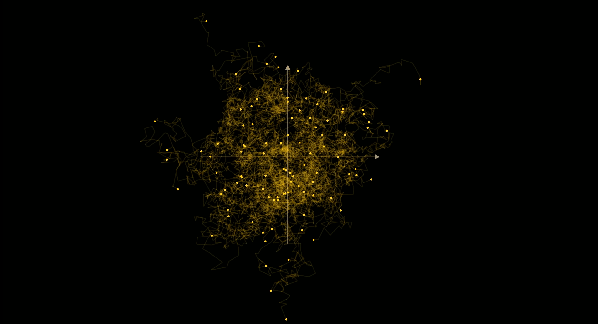
If we sample training data IID, then they will follow some structure in this space (real images follow some structure in the image space). For instance, in our toy example, let’s assume a spiral manifold.

Now, consider taking one training data sample from the manifold, and adding noise for a number of steps. This random walk depicts brownian motion, as can be seen from the image below.

Using this random walk, we then train a denoising network, asking it to undo all the noise. This seems like a huge task. How can we unlearn noise, which by definition is random?

The training data after adding noise looks like below, a bunch of random walks originating from the data manifold.

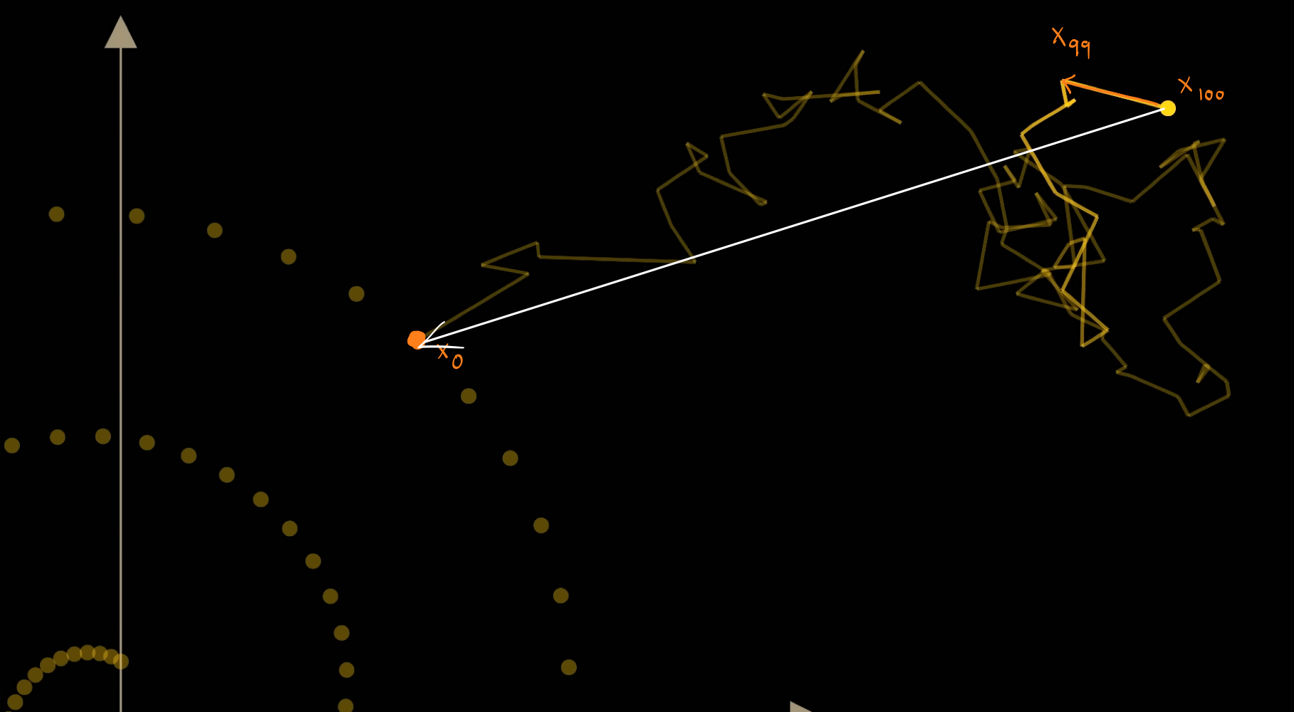
The key idea to understand is that, although the noise to add to go from $x_{100}$ to $x_{99}$ is completely random, it is biased towards the data manifold when we know the originating point $x_0$. The aggregate noise direction points towards the data manifold from which the random walk originated. 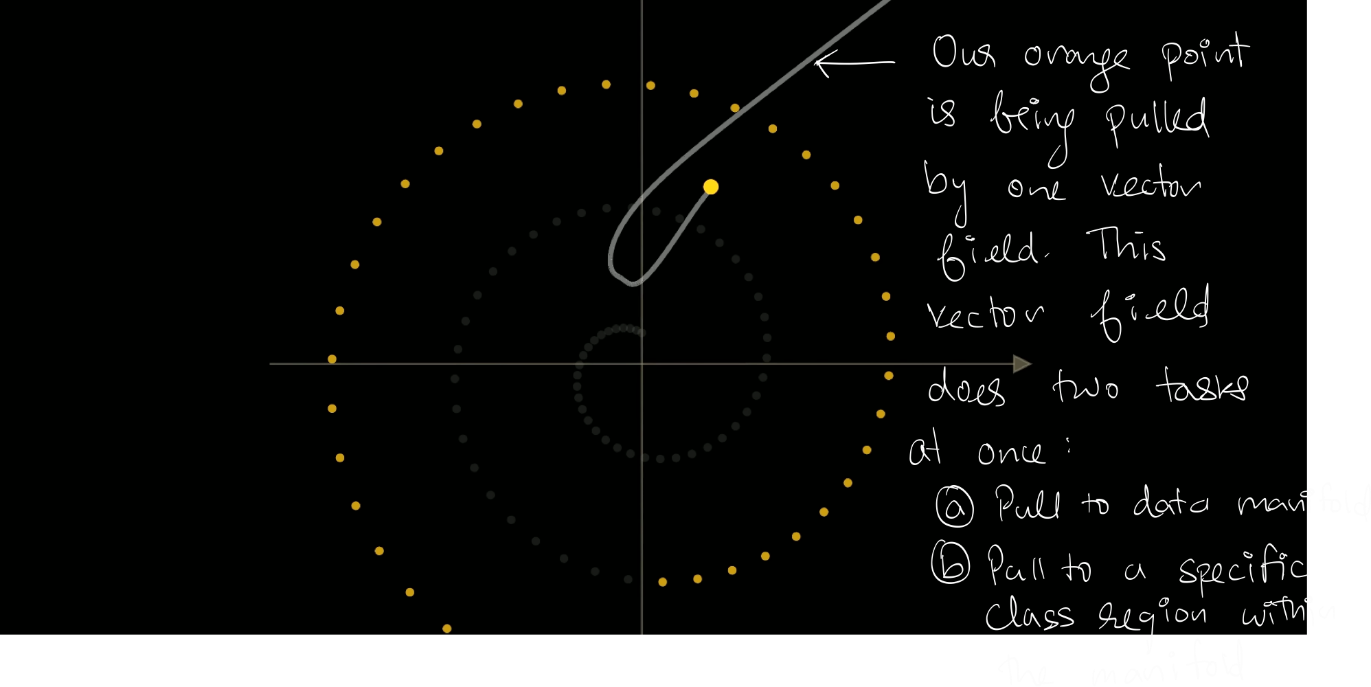Mathematically, we can show this: $$\mathbb{E}[x_{99} - x_{100} | x_0] = \frac{\mathbb{E}[x_{0} - x_{100} | x_0]}{100}$$ The model learns a vector field, that points towards the data manifold.

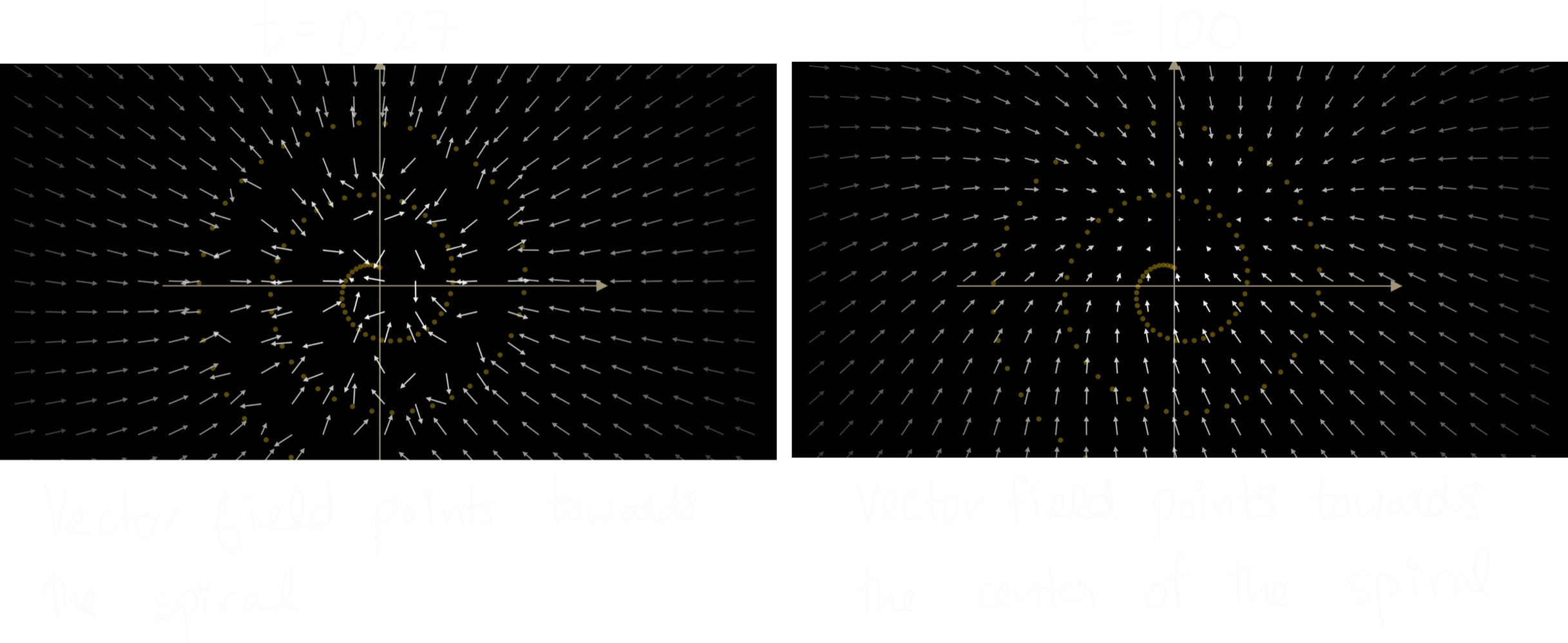
However, this vector field is for a noise at a fixed time t=100 (that is, 100 noise steps have been added to the original image). However, if you add noise to an image for only one time step, t=1, then the vector fields will point more towards the spiral.

The vector field for a given time t basically says if you were to take a random point in the image space, which direction should I move in to go to the most likely real image from the manifold. That is why points in the inner side of the outer spiral does not point towards the spiral itself but rather inside. This is because, if you take 100 steps of noise, from the outer spiral, you are more likely to be far away from it than that close.

Role of t: For larger t, the denoising model learns to denoise higher level structure. For smaller t, the model learns to denoise finer details of the image. At smaller t, the model operates close to the data manifold (I think?).

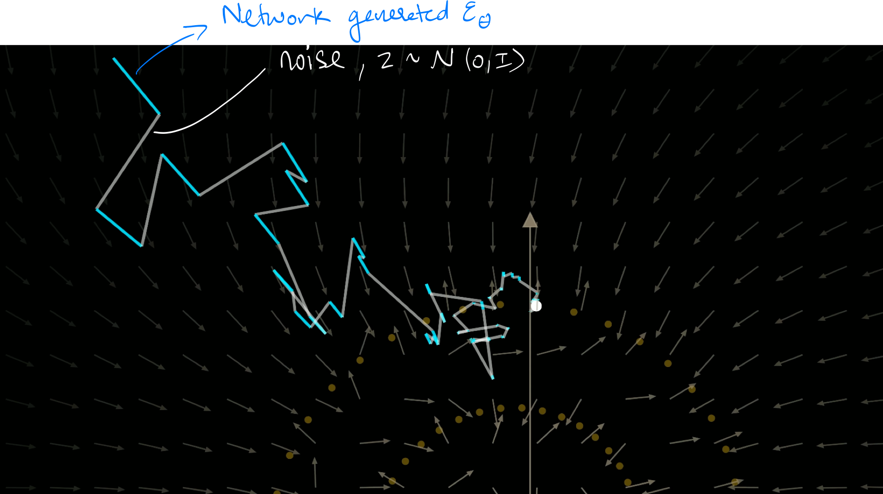
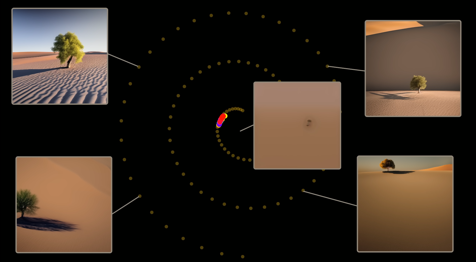
Finally, in the sampling process, we can see that we add an extra noise term from a gaussian after denoising it. This can seem counterintuitive. But without this, all the sampled points converge to the average of the data manifold by following the time-varying data manifolds.

Without the additional gaussian noise during sampling, we will converge at the average of the data manifold, leading to a more blurry image. As you can see in the example below, we get a blurry image of tree in a desert.

This is how the training and sampling algorithm looks like. During sampling, you can see that you add a random gaussian noise after denoising a step.

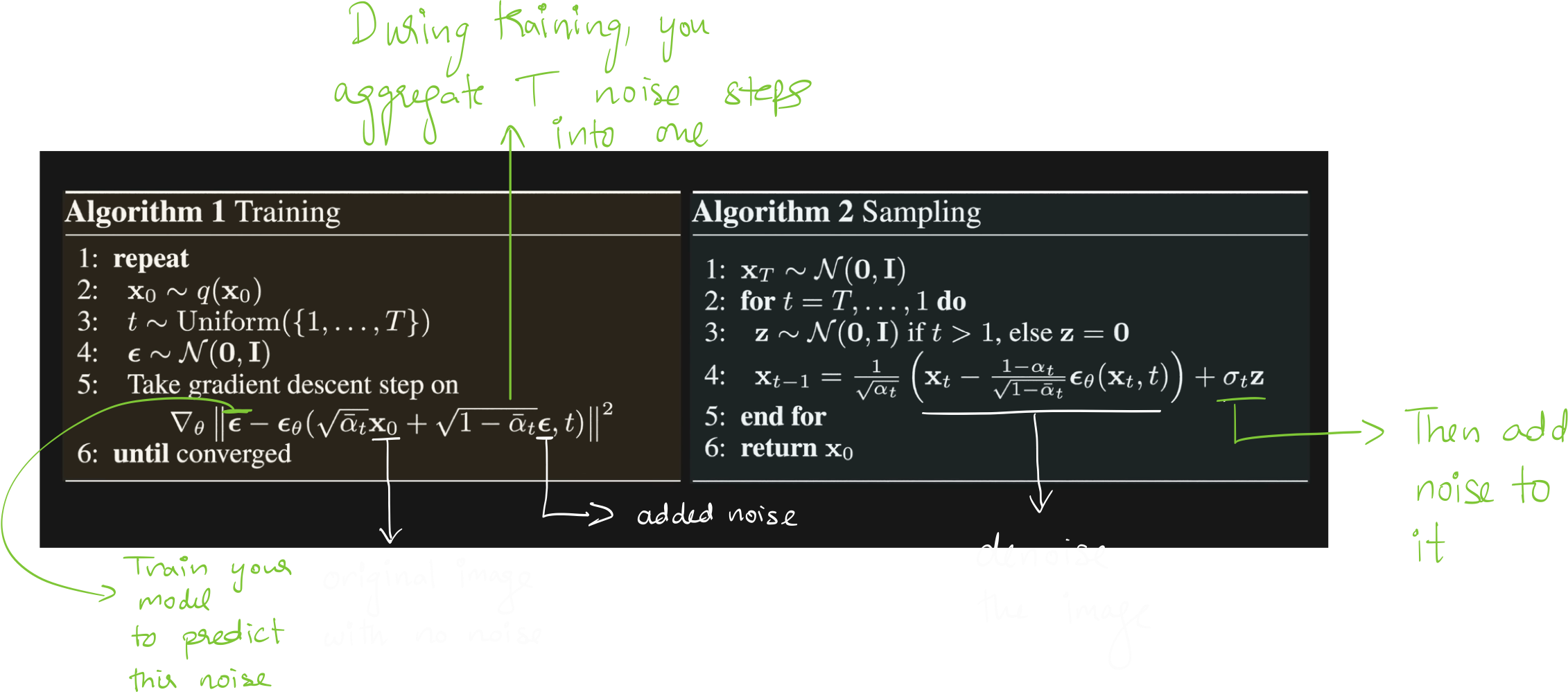
**As you can see, in the sampling process, you need to pass the input through the neural network for each step of denoising. This can be really expensive. **

How to guide the denoising process with a text prompt?

The core idea is to guide the denoising process using the text embedding output we get from Contrastive Language-Image Pretraining (CLIP) model.

One could pass the text embedding to the denoising neural network, and allow the model to learn to use the textual information to guide the denoising towards the right region of the data manifold.

The above example is when we include the text embedding as an input to the denoising network. What happens here is that we have one network that needs to drive the denoising process towards the data manifold, and at the same time, towards a specific region of the manifold, where the text embedding is present. However, often, the first aspect overdrives the second, leaving the final output stranded in between. Can we somehow decouple the two factors involved here?

The idea is to have two models: unconditional and conditional. You can use one model, and have a special no_class input to fuse both into one.

These two models are trained to do different things. The first model is simply trained to pull the points towards the data manifold in general. The second model is specifically trained to pull it to the class region within the data manifold.

When t is high (a lot of noise steps away from origin), both the models have a similar vector field. However, as t gets smaller (we get closer to the general data manifold), the conditional model points towards the class region within the data manifold, while the unconditional model simply drives the point towards the most likely origin on the data manifold.

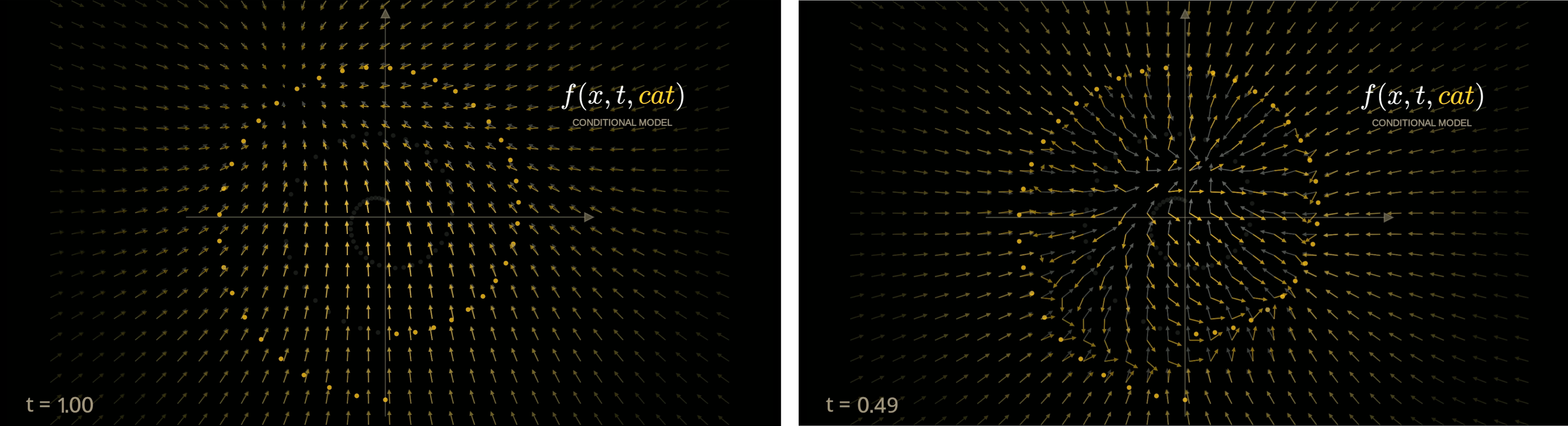
If you take the difference between the two vector fields, you can move towards the specific class region of the data manifold, and at the same time move away from the average.

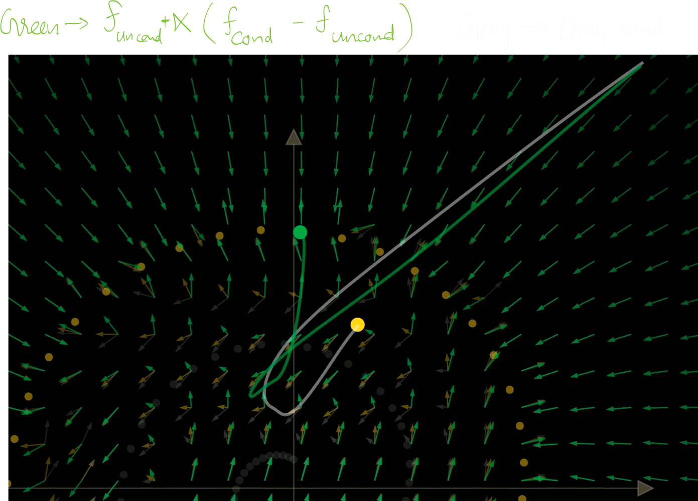
This method is called classifier free guidance.

Source

All images are taken from this excellent video by Welch Labs on 3blue1brown’s channel: https://www.youtube.com/watch?v=iv-5mZ_9CPY